November 7, 2026
Why GPU Performance Benchmarks
Are Not Deterministic
When benchmarking LLM inference on modern GPUs, we often focus on a single number: tokens per second.
For example, a B200 GPU running DeepSeek V4.1 Flash can deliver hundreds of thousands of output tokens per second in aggregate throughput under a particular serving configuration.
But what happens when you run the same benchmark multiple times? Do you get exactly the same number every time?
In practice, you may see noticeable differences, even when using the same GPU, model, and serving configuration.
Why?
When optimizing GPU kernels or AI inference systems, I often encounter this question. A performance improvement of 1% or 2% looks promising, but how do we know whether it’s a real improvement or simply benchmark noise?
We have well-established ways to improve benchmark consistency: warming up the GPU, controlling cache residency, locking GPU clocks, and repeating measurements. These practices help, but they don’t make GPU execution completely deterministic.
This raises an interesting question: Is the variation a benchmark problem, or is it simply how the hardware is designed to work?
In this post, I’d like to explore why CPU and GPU performance benchmarks are not always deterministic, where the variation comes from, and how we can distinguish measurement noise from a real performance improvement.
Is It a Bug or a Feature?
Could the variation be caused by a benchmark infrastructure bug that we should fix to make performance deterministic across runs?
As an engineer who strives for precision, I understand how frustrating nondeterministic results can be. However, I’ve learned throughout my career that not everything that initially appears unpredictable is necessarily a problem.
After graduating from college with a major in Microelectronics, I started my career in the Electronic Design Automation (EDA) industry, an interesting intersection of software and hardware.
Working as a field consultant at customer sites, I often encountered situations where people asked, “Is it a feature or a bug?”
Sometimes, unexpected behavior was simply a result of functionality that wasn’t well understood. Other times, it revealed previously undiscovered design flaws in corner cases.
I’d like to borrow this philosophy to understand what’s happening inside CPUs and GPUs.
Non-deterministic performance doesn’t always indicate a bug. Sometimes, it’s a result of how the hardware operates.
Let’s take a closer look.
1. How Do We Make GPU Benchmarks Reproducible?
Before investigating hardware-level nondeterminism, let’s review some common practices for setting up reliable GPU benchmarks.
Warm Up the GPU
GPU warmup is about more than stabilizing clock frequencies and temperatures.
The first few executions may trigger GPU initialization, memory allocation, kernel loading, autotuning, or JIT compilation. These operations introduce overhead that should be excluded from performance measurements.
Warmup should use the same workload configuration as the actual benchmark, followed by GPU synchronization before measurements begin.
For short-running kernels, the number of warmup iterations matters as well. A hundred executions of a short kernel might take only a few milliseconds, which may not be enough time for GPU clocks, power, and temperature to stabilize.
Control Cache Residency
Warmup introduces another complication: cache residency.
Repeatedly running the same kernel can leave data in the L2 cache, making subsequent executions faster than when data must be fetched from HBM.
One common technique is cache busting: accessing a buffer larger than the L2 cache before each measurement to evict previously cached data.
However, cache busting isn’t always desirable. If we’re measuring a workload that naturally benefits from data reuse, warm-cache performance may be more representative.
For example, KV cache behavior in an end-to-end LLM serving benchmark may depend heavily on cache residency.
The key is to understand what we’re trying to measure and configure cache behavior accordingly.
Lock GPU Clocks
GPU performance depends heavily on operating frequency. Fixing SM and memory clock frequencies helps reduce variability caused by dynamic frequency scaling.
However, clock locking alone doesn’t guarantee deterministic performance. Power and thermal limits can still affect actual operating frequencies.
We’ll come back to this when discussing hardware behavior.
Repeat Measurements
Finally, repeat measurements and examine their distribution rather than trusting a single result.
For kernel microbenchmarks, CUDA events help isolate GPU execution time from CPU launch overhead.
The median is useful for understanding typical performance, while the distribution and tail measurements tell us how inconsistent execution can become.
At this point, we’ve established several techniques to improve benchmark consistency:
- Warm up the GPU before collecting measurements.
- Control cache residency to understand memory behavior.
- Lock GPU clock frequencies when possible.
- Repeat measurements and analyze their statistical distribution.
Even with all these controls, performance still varies.
What went wrong?
2. Why Does GPU Performance Still Vary?
To understand why performance remains variable, we need to step beyond the software domain and look at how the hardware is designed to operate.
GPU Clocks, Power, and Temperature
Modern GPUs operate within predefined power and thermal limits. Under sustained workloads, hardware dynamically adjusts operating frequencies to remain within these limits.
Different workloads also have different power characteristics.
For example, a Tensor Core-intensive kernel can have very different power characteristics from a memory-intensive LLM decode kernel.
If a benchmark starts immediately after a long compute-heavy workload, the GPU may already be approaching its thermal or power limit.
Even with locked clocks, hardware protection mechanisms can reduce the actual operating frequency when necessary.
As a result, measured performance can still vary.
But what if power consumption and temperature are both stable? Should we then expect completely deterministic performance from CPUs and GPUs?
Not necessarily.
Caches and Memory Performance
Let’s revisit caches and the memory subsystem in GPUs and SoCs.
There are two broad categories of cache management: hardware-managed and software-managed caches.
When we run an application on a CPU or GPU, software instructions determine what executes and how it executes. However, many decisions inside the memory hierarchy are managed dynamically by hardware.
Cache replacement decisions, memory request ordering, and interference can change which data remains cached. As a result, memory latency and throughput may vary between executions.
HBM provides high bandwidth through multiple channels and banks operating in parallel. But high bandwidth doesn’t mean constant memory latency.
A memory request may hit an already-open DRAM row or require a different row to be activated. Memory-controller queue occupancy, read/write scheduling, and periodic refresh operations all affect service time.
As memory traffic increases, contention and queueing become more significant.
This matters particularly for memory-bandwidth-bound LLM decode workloads, especially at small batch sizes.
Even after controlling L2 cache residency and GPU clocks, we cannot guarantee identical HBM bank states or memory-controller conditions across benchmark runs.
The computation may be the same, but the memory system doesn’t necessarily behave the same way.
This is one reason why GPU performance can be nondeterministic by design.
GPU Scheduling and Resource Contention
A GPU contains several built-in hardware scheduling mechanisms that manage execution across streaming multiprocessors (SMs).
Since GPU execution is highly parallel, the exact ordering and timing of operations are not necessarily guaranteed to be identical across runs.
Warp scheduling depends on instruction readiness and available resources. Small differences in memory response timing can affect when dependent instructions become eligible for execution.
Concurrent kernels can also compete for SM resources, cache capacity, and memory bandwidth.
For multi-GPU workloads, communication and synchronization introduce additional dependencies. A delay on one GPU can leave other GPUs waiting at a collective operation.
These effects become particularly important when moving from isolated kernel benchmarks to full inference systems.
3. Why Is AI Inference Even More Variable?
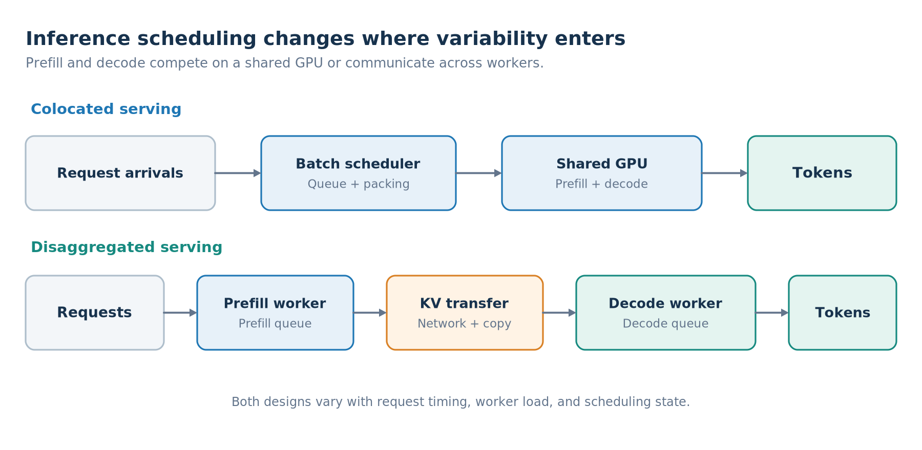
LLM serving systems introduce another layer of complexity: dynamic workloads, scheduling decisions, and queueing at the cluster level.
Even if the underlying GPU hardware behaves consistently, the workload presented to it may change from one execution to another.
Continuous Batching and Batch Size
Inference runtimes dynamically add and remove requests from batches.
Even with the same overall request arrival rate, slightly different arrival times can change batch composition and kernel execution sequences.
This affects GPU utilization, throughput, and individual request latency.
Larger decode batches and speculative decoding can improve weight reuse and increase arithmetic intensity, potentially shifting workloads from memory-bandwidth-bound to compute-bound behavior.
However, KV cache traffic can still be a bottleneck, particularly at long context lengths.
Both techniques affect throughput and per-token latency. The benefits of speculative decoding may also diminish when compute resources are already saturated.
Prefill and Decode Interference
When prefill and decode share the same GPU, a long prefill request can delay decode iterations for existing users, increasing inter-token latency (ITL).
Chunked prefill and decode-priority scheduling help manage this interference, but they introduce tradeoffs between time to first token (TTFT) and time per output token (TPOT).
The resulting performance depends not only on the workload itself but also on how requests are scheduled and interleaved.
Disaggregated Serving
Disaggregated inference separates prefill and decode onto different GPU workers, reducing direct competition between the two phases.
However, it doesn’t eliminate performance variability. Instead, it introduces new dependencies, including KV cache transfers, network contention, worker load balancing, and scheduling queues.
A slow KV-cache transfer can delay TTFT or, if the first token is already returned, widen the gap before the second token, while uneven decode-worker utilization can affect ITL.
Disaggregation changes where the bottlenecks occur rather than making performance deterministic.
Queueing Near Saturation
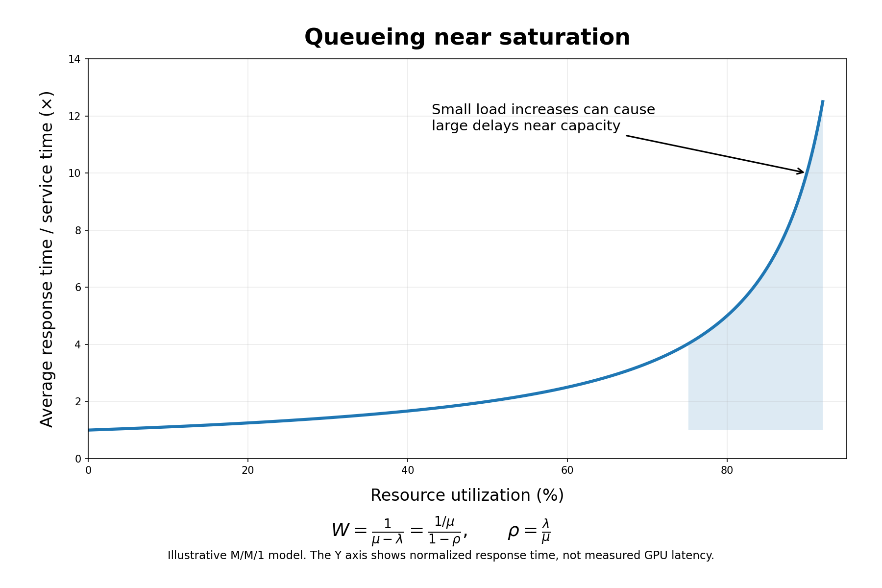
As an inference server approaches its maximum sustainable throughput, small differences in request arrival times can produce much larger latency differences.
A simplified decomposition of TTFT is:
TTTFT = Trequest overhead + Tqueue + Tprefill
Some operations can overlap, but this model illustrates the major sources of latency variability.
As offered traffic approaches the server’s capacity, queueing delays become increasingly sensitive to small differences in request arrival and service times.
The same hardware can therefore produce very different TTFT distributions under different request arrival patterns.
This is why measuring maximum token throughput alone is insufficient when evaluating an inference server.
We also need to understand how latency behaves under load. A server may deliver excellent average throughput while some users experience much slower responses.
4. How Much Benchmark Noise Should We Expect?
This is probably the most practical question. What percentage improvement can we confidently consider a real performance gain?
In practice, I would consider a 1% improvement potential noise. A 2% improvement may still be within the noise range. What about 3%?
I don’t think there is a straightforward answer. It depends on the workload, benchmark methodology, and execution environment.
A recent study by Olympio et al., Reproducible LLM Inference Benchmarking: A Sequential Isolation Protocol for Regression Testing (October 2026), evaluated 144 model, context-length, and concurrency configurations.
By improving benchmark controls, the researchers reduced the average coefficient of variation (CV) for repeated P50 TTFT measurements from 15.2% to 2.2%.
That’s a substantial improvement.
However, these results describe end-to-end inference serving benchmarks, not the intrinsic measurement noise of isolated GPU kernel execution.
Different benchmarks have fundamentally different characteristics.
An isolated GPU kernel may achieve very consistent execution times under controlled conditions.
End-to-end inference introduces additional sources of variation, including CPU overhead, runtime scheduling, memory management, and communication.
Online serving adds another layer of complexity through changing request arrivals and queueing behavior.
I wouldn’t assume a fixed acceptable noise threshold.
I would also look beyond average performance. An optimization that improves mean throughput but worsens tail latency may not be beneficial for an interactive inference service.
The metrics should match what we’re trying to optimize:
- GPU kernel: Execution time, cache behavior, and hardware utilization.
- Inference runtime: Kernel launch overhead, scheduling, batching, and memory management.
- Online serving: Throughput, TTFT, ITL, and tail latency across different load levels.
Workload consistency matters too.
Different prompt lengths, MoE expert-routing patterns, or speculative-decoding acceptance rates can change the amount of actual computation.
These workload differences shouldn’t be confused with measurement noise.
Ultimately, determining whether a performance improvement is real requires understanding both the variability of the benchmark and the behavior of the workload being measured.
5. Final Thoughts
GPU benchmarking looks simple until you’re trying to prove a small performance improvement.
Warmup, cache control, locked clocks, and repeated measurements help, but they can’t completely eliminate the effects of dynamic hardware and runtime behavior.
For AI inference, the problem becomes more complicated as we add continuous batching, prefill/decode scheduling, distributed execution, and queueing.
Some variability is measurement noise we should minimize. Other variability is real system behavior that we need to understand.
For me, the goal isn’t to make every benchmark run produce exactly the same number.
It’s to understand why the numbers change and whether an optimization actually improves performance.
After all, a performance improvement is only useful if we can demonstrate that it is real.