Memory Bandwidth, Throughput, and Latency: What Really Limits Performance?

Frontier AI workloads rely heavily on both CPUs and GPUs, and memory performance plays a major role in how efficiently these systems run. As AI models continue to grow, memory bandwidth often gets much of the attention. But bandwidth alone doesn’t tell us how well a system will perform.

In this post, I’d like to revisit three closely related concepts: memory bandwidth, throughput, and latency, and explore how they affect real-world performance.

Imagine a compute core issuing a memory request that misses in its local caches and cannot be satisfied by another cache. The request must be serviced by DRAM, traveling through the on-chip interconnect to a memory controller before the data eventually returns to the core.

When the system is lightly loaded, the request can move through the memory hierarchy with little contention.

Now imagine hundreds of cores issuing requests at the same time. They compete for interconnect links, buffers, and memory controllers. Some requests wait for arbitration, others encounter busy DRAM banks, and queues start building up.

The memory interface hasn’t changed, but the time it takes to complete a request can be very different.

This is the kind of problem I worked on while developing the Scalable Coherent Fabric (SCF) architecture for Intel Xeon data center CPUs. In a multi-core, multi-die system, we needed to understand how requests moved between cores, caches, and memory, and how routing, arbitration, and congestion affected performance.

I still remember my manager at Intel, a Senior Principal Architect, who often reminded us: “Latency is king.”

That lesson has stayed with me as my work expanded from CPU interconnects to GPU architecture and AI inference.

For hardware architects, the question is: How do we design memory systems that deliver not only high peak performance, but also predictable performance under real workloads?

For software engineers, there’s a related question: Given a particular workload and hardware architecture, what’s the realistic upper bound on achievable performance?

1. Memory Bandwidth: Theoretical Data Transfer Capacity

Memory bandwidth describes the rate at which data can be transferred through a memory interface.

For DRAM, theoretical peak bandwidth depends on the data transfer rate and the aggregate width of the memory interfaces.

BW_peak = (R_data × W_bus) / 8

Where:

• R_data is the data transfer rate in transfers per second per pin.
• W_bus is the aggregate data bus width in bits.
• Division by 8 converts bits to bytes.

Let’s use LPDDR6 as an example.

Consider an LPDDR6 system with eight 24-bit channels running at 14,400 MT/s.

The total interface width is:

W_bus = 8 × 24 = 192 bits

The theoretical raw bandwidth is:

BW_raw = (14,400 × 10⁶) × 192 / 8 = 345.6 × 10⁹ bytes/s = 345.6 GB/s

That’s an impressive number, but it doesn’t mean applications can transfer 345.6 GB of useful data every second.

Each 24-bit LPDDR6 channel comprises two 12-bit subchannels. A BL24 transfer on one subchannel carries 288 physical bits. Assuming 256 bits of useful data and 32 additional bits for metadata and other interface functions, the payload efficiency is:

η_payload = 256 / 288 = 8 / 9

The corresponding theoretical payload bandwidth is:

BW_payload = 345.6 × 8 / 9 = 307.2 GB/s

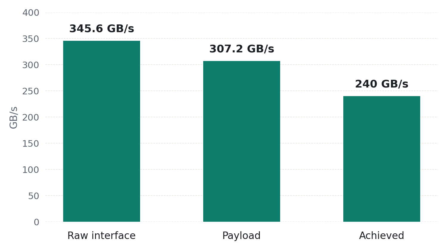
We now have two different bandwidth numbers: 345.6 GB/s of raw interface bandwidth and 307.2 GB/s of theoretical payload bandwidth.

Neither guarantees what an application will actually achieve.

2. Throughput: How Much Data Actually Gets Through?

Suppose an application running on this LPDDR6 system sustains 240 GB/s of useful memory traffic.

Its effective bandwidth utilization is:

η = 240 / 307.2 × 100% ≈ 78.1%

What limits the achieved throughput?

Some of the difference comes from DRAM timing constraints. Row activation, precharge, refresh, and read/write turnaround all consume cycles.

Memory access patterns also matter.

Sequential accesses with good row locality are generally easier for the memory controller to schedule efficiently. Random accesses with frequent row conflicts can reduce throughput.

Bank-level parallelism matters too. If requests are distributed across independent banks, the controller has more opportunities to overlap memory operations. If many requests target the same bank, some operations must wait.

Another factor is memory-level parallelism. Even a high-bandwidth memory interface can sit idle if the processor doesn’t generate enough outstanding requests.

And then there’s the interconnect.

In a multi-core CPU, a memory controller may have available bandwidth while some cores are still stalled waiting for data. The bottleneck could be an interconnect link, an arbitration point, or a shared queue somewhere between the core and memory.

Available DRAM bandwidth doesn’t necessarily mean the same bandwidth is available end to end.

This distinction is also important when optimizing software.

If a kernel achieves only 60% of theoretical memory bandwidth, it doesn’t automatically mean the remaining 40% can be recovered through software optimization.

The workload may not have enough independent memory requests. Its access pattern may cause frequent row conflicts. Or another part of the system may already be saturated.

Before trying to improve throughput, we need to understand what’s limiting it.

3. Latency: Why More Bandwidth Doesn’t Always Help

Bandwidth tells us how much data can move per second. Latency tells us how long we wait for a particular request to complete.

For a cache miss that must be serviced by external memory, we can think of the total latency as:

L_total = L_network + L_queue + L_controller + L_DRAM + L_return

This is a simplified breakdown. Some operations may overlap, and the actual path depends on the architecture.

Let’s compare two situations.

In a lightly loaded system, a request moves through the interconnect without much contention. The memory-controller queue is short, and DRAM can service the request with little waiting.

In a heavily loaded system, many cores and accelerators compete for the same resources. Requests may wait in interconnect queues, at arbitration points, or inside the memory controller.

The LPDDR6 interface still operates at the same data rate, but the observed request latency can be much higher.

Much of the increase can come from queueing delay. Contention can also change how requests are scheduled and serviced, for example, by changing row locality or introducing additional read/write turnarounds.

This is why I like to distinguish between unloaded latency and loaded latency.

Unloaded latency gives us a baseline for the architecture. Loaded latency tells us what happens when real workloads compete for shared resources.

Both are important, but loaded latency is often where architectural bottlenecks become visible.

4. What Happens When the System Approaches Saturation?

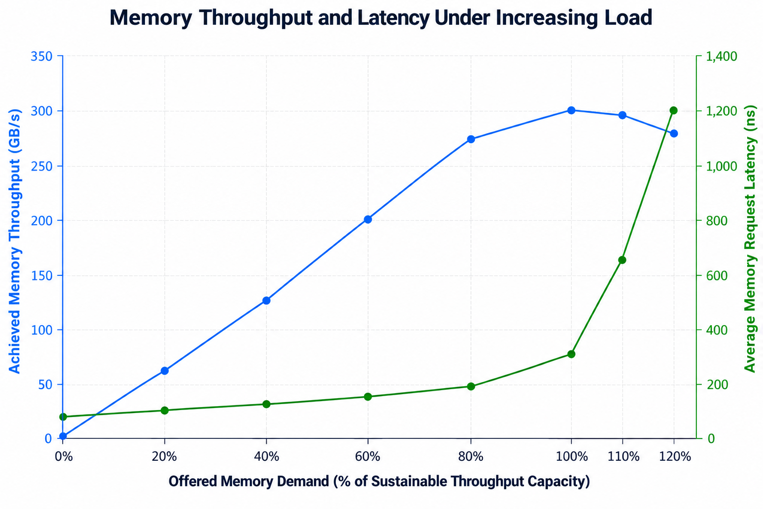
As memory traffic increases, throughput and latency behave differently.

At low traffic levels, increasing the request rate usually increases throughput without significantly changing latency.

As traffic grows, shared resources become busier and requests spend more time waiting.

Eventually, the system approaches its sustainable throughput limit.

Near that point, sending more requests produces diminishing throughput gains. Instead, queueing delays increase, and latency can rise sharply. In a real system, finite buffers and backpressure eventually limit how many additional requests can enter.

This was an important consideration in our interconnect performance modeling.

The workload’s traffic pattern also makes a difference.

Consider two applications running on the same memory subsystem.

One generates sequential reads with good row locality and enough independent requests to keep memory busy.

The other generates random accesses with frequent row conflicts and dependencies between requests.

Both are memory-intensive, but they can achieve very different throughput and latency.

When evaluating a design, I want to see how throughput and latency change as offered traffic increases, and where the system begins to saturate.

The saturation point matters because it tells us how much traffic the system can sustain before additional load starts causing significant delays.

For many workloads, operating near maximum throughput may not be the best choice if it causes excessive latency.

5. Memory-Level Parallelism: Connecting Bandwidth and Latency

Bandwidth and latency are tied together by a third quantity: the number of memory requests outstanding at any moment.

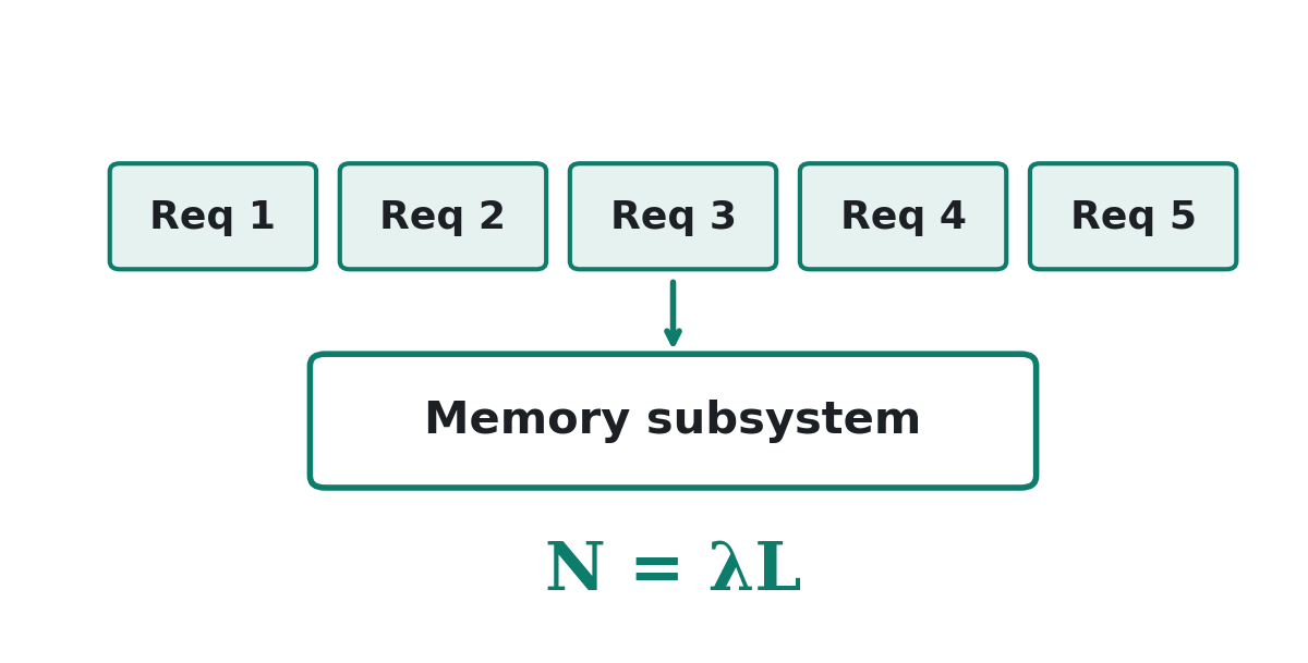
Little’s Law gives us:

N = λL

Where:

• N is the average number of outstanding requests.
• λ is the completed request rate.
• L is the average request latency.

Let’s return to our LPDDR6 example.

Suppose the system sustains 240 GB/s, with an average request latency of 100 ns.

For simplicity, assume each completed request transfers 64 useful bytes.

The completed request rate is:

λ = (240 × 10⁹) / 64 = 3.75 × 10⁹ requests/s

Applying Little’s Law:

N = 3.75 × 10⁹ × 100 × 10⁻⁹ = 375

Assume a stable workload, and measure both outstanding requests and latency over the same path from request admission to completion. Also assume that each completion accounts for 64 bytes of the traffic used in the bandwidth calculation.

Under these assumptions, sustaining 240 GB/s at an average latency of 100 ns corresponds to an average of 375 requests in flight across the measured system.

A workload that issues one dependent memory request at a time may spend most of its time waiting, even when the memory interface is far from saturated.

A workload with hundreds of independent requests can overlap those accesses and achieve much higher throughput.

But increasing concurrency also creates more competition for shared resources. At some point, additional requests contribute more to queueing than useful throughput.

Finding that balance is an important part of architecture design.

6. What Should We Measure?

I’d want to understand a memory subsystem’s unloaded latency, sustainable throughput, latency under load, and how performance changes with request concurrency and access patterns.

I’d also want to know where the bottleneck appears first.

Is it the DRAM interface? A memory-controller queue? An interconnect link? Or is the workload simply unable to expose enough parallelism?

These questions matter for both hardware and software optimization.

Without understanding the bottleneck, it’s easy to spend time improving something that isn’t limiting performance.

7. Why This Matters for AI Inference

AI inference is a good example of why bandwidth, throughput, and latency need to be considered together.

Different phases of large language model inference can have very different performance characteristics.

Prefill processes multiple input tokens in parallel, often creating substantial matrix multiplication workloads. Depending on batch size, model dimensions, and hardware utilization, performance may be limited by compute throughput or memory bandwidth.

Decode, particularly at small batch sizes, is often limited by the bandwidth needed to read model weights and KV-cache data. At larger batch sizes or longer context lengths, the bottleneck can shift.

But memory bandwidth doesn’t explain every performance problem.

Irregular memory accesses, synchronization dependencies, cache misses, and insufficient outstanding requests can expose latency even when the memory subsystem still has available bandwidth.

This is where hardware architecture and software optimization need to work together.

Architects need to understand how memory controllers, interconnects, caches, and scheduling mechanisms behave under load.

Software engineers need to understand how tensor layouts, batching, kernel fusion, memory access patterns, and execution scheduling affect the traffic generated by the workload.

The goal isn’t simply to maximize peak bandwidth. It’s to achieve high useful throughput while keeping latency under control for the workloads that matter.

Final Thoughts

Peak bandwidth describes a transfer ceiling. Achieved memory throughput describes the rate sustained by a particular workload. Latency describes the time individual requests spend in the system.

None of these tells the whole story alone. To understand performance, we also need to know where traffic is measured, how much concurrency the workload exposes, and how shared resources behave under load.

In future posts, I’ll apply these ideas to GPU architecture and AI inference, where memory behavior, execution scheduling, and workload concurrency introduce additional performance challenges.